Real case

Note

In this section, indices enable to number the nodes in a layer (example: \(a_j\) is the \(j\)-th node of the last layer which has \(n_j\) nodes).

A forward neural network transform an input \(x\) composed by \(n_i\) components \(x_i\) into an output layer \(j\) composed by \(n_j\) components \(a_j\). Between those, several hidden layers are found. An example in the training data is composed by a pair \((x, y)\): an input and a target. A target is composed by \(n_j\) components \(y_j\) (same number as the output layer).

Every layer can have a different number of nodes. The figure Real case FNN (basecase) shows this graph. Many edges, weights and biases are omitted for clarity. Every node of each layer is actually connected to every node of the next. The dashed lines on the right symbolize a comparison between the output layer \(j\) and the training target \(y\). The dotted lines indicate the index of nodes inside a layer.

Focusing on the last layer \(j\), the only weight and bias which appear are the weight \(w_{jk}\) between nodes \(a_k\) and \(a_j\) and the bias \(b_j\) of node \(a_j\). The goal is to be able to compute the gradients of the loss function with respect to \(w_{jk}\) and \(b_j\). These gradients will be used in the gradient descent algorithm to optimize these weights and biases in order to minimize the loss function over all the training examples. Let us use \(t\) as the index for the \(n_t\) training example pairs \((x, y)_t\).

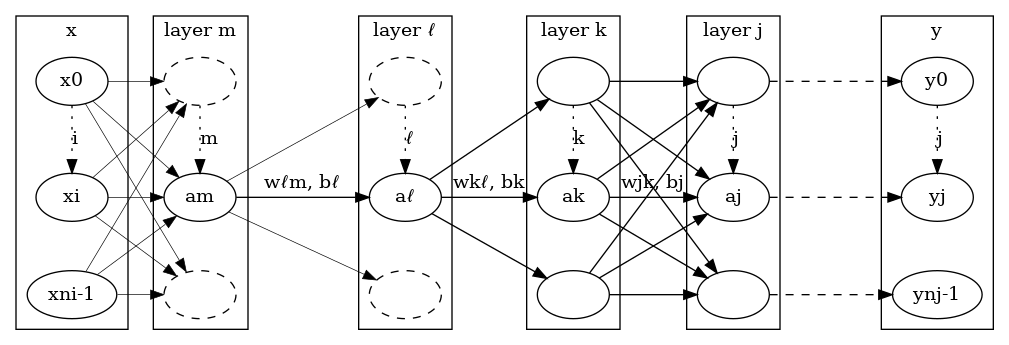
Real case FNN - (basecase)

Regression

Similarly to the simple case, the cost \(J\) is shown in equation (1) from the comparison of the training targets to all the predictions made by the network. As mentioned, the simplest cost for regression is the average norm 2 of the difference between training targets and estimations.

(1)\[ J = \cfrac{1}{n_t} \sum _t \cfrac{1}{2} \sum _j (a_{jt} - y_{jt})^2\]

For clarity, the averaging over \(t\) will be dropped for the time being. Since the gradient of a sum is the sum of the gradients, let us write down the equation for a single training example, then at the very end, the averaging over training data will be seamlessly reintroduced.

(2)\[ J = \cfrac{1}{2} \sum _j (a_{j} - y_{j})^2\]

A value of the node \(a_j\) is obtained in two steps from all the values of the previous layer nodes \(a_k\). First one obtains the intermediate variable \(z_j\) using the weights \(w_{jk}\) and bias \(b_j\) of the edge leading to the node \(a_j\) from the \(k\) layer, then the activation function \(\sigma(z_j)\) is used, see equations (3):

(3)\[\begin{split}z_j &= b_j + \sum_k w_{jk} \cdot a_k \\ a_j &= \sigma(z_j)\end{split}\]

The derivation chain rule is applied to compute the gradient terms for the last layer, see equations (3) and (4). The equations are the same as the Simple case because only a single term of the sum has a \(w_{jk}\) term in it for a specific value of \((j, k)\) as illustrated in figure Real case FNN - (w_jk).

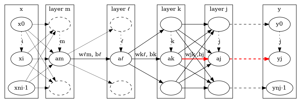
Real case FNN - (\(w_{jk}\))

(4)\[\begin{split} \cfrac{\partial J}{\partial w_{jk}} &= \left( \cfrac{\partial J}{\partial a_j}\cfrac{\partial a_j}{\partial z_j} \right) \cfrac{\partial z_j}{\partial w_{jk}} \\ &= \underbrace{ \left( (a_j - y_j)\cdot \overbrace{\sigma'(z_j)}^{=1 \textrm{ if linear last layer}} \right) }_{ \cfrac{\partial J}{\partial z_j} } \cdot a_k\end{split}\]

(5)\[\begin{split} \cfrac{\partial J}{\partial b_j} &= \cfrac{\partial J}{\partial z_j} \cfrac{\partial z_j}{\partial b_j} \\ &= \cfrac{\partial J}{\partial z_j} \cdot 1\end{split}\]

To obtain the node \(a_k\) from all the nodes \(a_{k\ell}\):

(6)\[\begin{split}z_k &= b_k + \sum_{\ell} w_{k\ell} \cdot a_{\ell} \\ a_k &= \sigma(z_k)\end{split}\]

The derivation chain rule is also applied to compute the gradient terms for the second to last layer, see equations (7) and (8). However, as illustrated in figure Real case FNN - (w_kl), this time all the nodes \(a_j\) are affected by a change in \(w_{k\ell}\) and a summation is required.

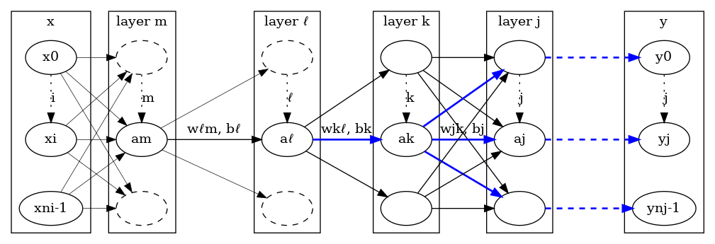
Real case FNN - (\(w_{k\ell}\))

(7)\[\begin{split} \cfrac{\partial J}{\partial w_{k\ell}} &= \sum_j \cfrac{\partial J}{\partial z_j} \left( \cfrac{\partial z_j}{\partial a_k}\cfrac{\partial a_k}{\partial z_k} \right) \cfrac{\partial z_k}{\partial w_{k\ell}} \\ &= \underbrace{ \left( \sum_j \cfrac{\partial J}{\partial z_j} \cdot \left( w_{jk} \cdot\sigma'(z_k) \right) \right) }_{ \cfrac{\partial J}{\partial z_k} } \cdot a_{\ell}\end{split}\]

(8)\[\begin{split} \cfrac{\partial J}{\partial b_k} &= \cfrac{\partial J}{\partial z_k} \cfrac{\partial z_k}{\partial b_k} \\ &= \cfrac{\partial J}{\partial z_k} \cdot 1\end{split}\]

From this point, the method should seem straightforward. Equation (7) shows how to obtain the sensitivity \(\cfrac{\partial J}{\partial z_k}\) of the cost to a variation of \(z_k\) from the sensitivities of the forward next layer \(\cfrac{\partial J}{\partial z_j}\). This step is repeated from right to left to compute the cost gradient component for every weight and bias.

For example, the next step is to obtain the gradient terms relative to the \(\ell\) layer. Figure Real case FNN - (w_lm) shows that a change in the \(w_{\ell m}\) coefficients impacts the values of all nodes of all forward layers. However, the sensitivities \(\cfrac{\partial J}{\partial z_k}\) are already known. The main task is only to obtain the \(\cfrac{\partial J}{\partial z_\ell}\) from them, see equations (9) and (10).

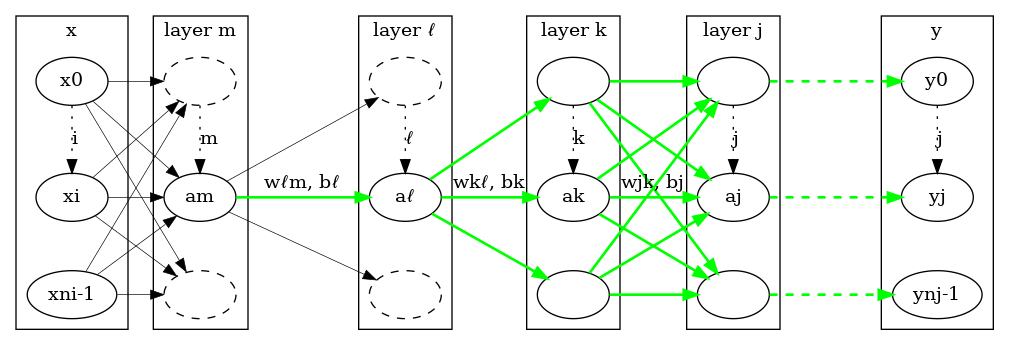
Real case FNN - (\(w_{\ell m}\))

(9)\[\begin{split} \cfrac{\partial J}{\partial w_{\ell m}} &= \sum_k \cfrac{\partial J}{\partial z_k} \left( \cfrac{\partial z_k}{\partial a_\ell}\cfrac{\partial a_\ell}{\partial z_\ell} \right) \cfrac{\partial z_\ell}{\partial w_{\ell m}} \\ &= \underbrace{ \left( \sum_k \cfrac{\partial J}{\partial z_k} \cdot \left( w_{k\ell} \cdot\sigma'(z_\ell) \right) \right) }_{ \cfrac{\partial J}{\partial z_\ell} } \cdot a_{m}\end{split}\]

(10)\[\begin{split} \cfrac{\partial J}{\partial b_\ell} &= \cfrac{\partial J}{\partial z_\ell} \cfrac{\partial z_\ell}{\partial b_\ell} \\ &= \cfrac{\partial J}{\partial z_\ell} \cdot 1\end{split}\]

Once all the gradients components are calculated, they must be averaged on several inputs to form a correction for the gradient descent.

Multi-class classification

For multi-class classification, even if the loss function seems very different, the final expression for the gradient is very similar. With the loss function for a single training example, a single non zero term corresponding to the correct class in the following sum:

(11)\[ \begin{align}\begin{aligned}J &= - \sum_{j} y_{j} \ln(a_{j})\\ &= - \ln(a_{j=j^*})\end{aligned}\end{align} \]

With \(j^*\) the index of the correct class, the chain rule for the last layer is:

(12)\[\begin{split} \cfrac{\partial J}{\partial w_{jk}} &= \left( \cfrac{\partial J}{\partial a_j}\cfrac{\partial a_j}{\partial z_j} \right) \cfrac{\partial z_j}{\partial w_{jk}} \\ &= \left( \left(- \cfrac{1}{ a_{j=j^*}} \right) \cdot a_{j=j^*} (y_{j=j^*}-a_{j=j^*}) \right) \cdot a_k \\ &= \underbrace{ \left( a_{j=j^*} - y_{j=j^*} \right)}_{\cfrac{\partial J}{\partial z_j}} \cdot a_k\end{split}\]

This expression is similar as the one obtained for regression for a linear last layer.

Note

Both for regression or multi-class classification, the gradient is null when the estimation meets the target exactly: if the prediction is perfect, no need for a correction.

Hint

Concerning the implementation of these type of expression:

• try to identify matrix multiplication disguised in index notation. (then use dot)

• remember that you can always transpose a matrix if the summation is carried along the row index.

• take advantage of numpy element-wise operations.

• take advantage of numpy broadcasting rules.

• a 1d array can be converted into a 2d array with one size equal to 1 using np.newaxis.

Exercise (easy)

Lower case symbols are 1d array; upper case symbols are 2d array. Implement concisely the following equations (use non square 2d arrays):

1. \(w_i = u_i v_i\)

2. \(v_i = \sum_j u_j A_{ij}\)

3. \(v_j = \sum_i u_i A_{ij}\)

4. \(B_{ij} = A_{ij} u_j\)

5. \(B_{ij} = A_{ij} u_i\)

6. \(A_{ij} = u_i v_j\)

Correction

src

"""few examples of basics numpy operations:
+ element wise
+ matrix
+ broadcast"""

import numpy as np


# 1
u = np.array([1, 2])
v = np.array([3, 4])
w = u * v  # element-wise
print(u, v, w, "\n", sep="\n")

# 2
A = np.array([[1, 2], [3, 4], [5, 6]])
u = np.array([1, 2])
v = A.dot(u)  # matrix
print(A, u, v, "\n", sep="\n")

# 3
A = np.array([[1, 2], [3, 4], [5, 6]])
u = np.array([1, 2, 3])
v = A.T.dot(u)
print(A, u, v, "\n", sep="\n")

# 4
A = np.array([[1, 2], [3, 4], [5, 6]])
u = np.array([1, 2])
B = A * u  # broadcast
print(A, u, B, "\n", sep="\n")

# 5
A = np.array([[1, 2], [3, 4], [5, 6]])
u = np.array([1, 2, 3])
B = (A.T * u).T  # broadcast
print(A, u, B, "\n", sep="\n")

# 6
u = np.array([1, 2])
v = np.array([3, 4, 5])
A = v * u[:, np.newaxis]  # broadcast
Abis = u[:, np.newaxis].dot(v[np.newaxis, :])
print(u, v, A, Abis, "\n", sep="\n")

Exercise (difficult)

1. How would you calculate \(\cfrac{\partial a_j}{\partial x_i}\) (first, for a single \(j, i\) pair, then for any \(j\) and a given \(i\))? How to generalize to the entire jacobian (any \(j, i\))?

2. Draw by hand the shape of every operation required to implement the jacobian with matrix product, transpose and broadcast.

3. Analyze the following code and map every operation to the previous question.

src

    def jacobian(self, input_: Vector) -> Array2D:
        self.infer(input_)
        jacobian: Array2D = np.eye(self.nb_nodes_per_layer_including_input[0])
        for ind_layer in range(0, self.nb_layers):
            layer, _, activation_derivative = (
                self.get_layer_activation_activation_derivative(ind_layer)
            )
            jacobian = (
                layer.weights.dot(jacobian).T
                * activation_derivative(layer.z)  # broadcast
            ).T

        return jacobian

Correction

\[\begin{split}\cfrac{\partial a_j}{\partial x_i} &= \cfrac{\partial a_j}{\partial z_j} \sum _k \cfrac{\partial z_j}{\partial a_k} \cfrac{\partial a_k}{\partial x_i} \\ &= \sigma'(z_j) \sum _k w_{jk} \cfrac{\partial a_k}{\partial x_i} \\ &= \sigma'(z_j) \sum _k w_{jk} \sigma'(z_k) \sum _l w_{kl} \cfrac{\partial a_l}{\partial x_i}\\ &= \sigma'(z_j) \sum _k w_{jk} \sigma'(z_k) \sum _l w_{kl} \sigma'(z_l) \sum _m w_{lm} \cfrac{\partial a_m}{\partial x_i}\end{split}\]

When reaching the first layer, the \(\cfrac{\partial a_m}{\partial x_i}\) is simpler:

\[\begin{split}\cfrac{\partial a_m}{\partial x_i} &= \cfrac{\partial a_m}{\partial z_m} \cfrac{\partial z_m}{\partial x_i} \\ &= \sigma'(z_m) w_{mi}\end{split}\]

As a result, if an inference has been performed for a given input \(x\), then all the \(z\) and \(a\) are up to date. Then, the calculation looks a little like an inference:

\[\begin{split}\cfrac{\partial a_m}{\partial x_i} = \sigma'(z_m) w_{mi} &~ \textrm{which is a vector varying } m \\ \sum _m w_{lm} \cfrac{\partial a_m}{\partial x_i} &~ \textrm{ is a product between weight matrix and the previous vector } \\ \sigma'(z_l) \sum _m w_{lm} \cfrac{\partial a_m}{\partial x_i} &~ \textrm{can be obtained with a broadcast of the activation derivative vector } \\ \sum _l w_{kl} \cfrac{\partial a_l}{\partial x_i} &~ \textrm{ is a product between weight matrix and the previous vector }\end{split}\]

One can just as easily obtain the full jacobian matrix if one considers the first line as a matrix for all \(m\) and \(i\). When only linear activation functions are used, the gradient is logically found to be the product of every weight matrices.

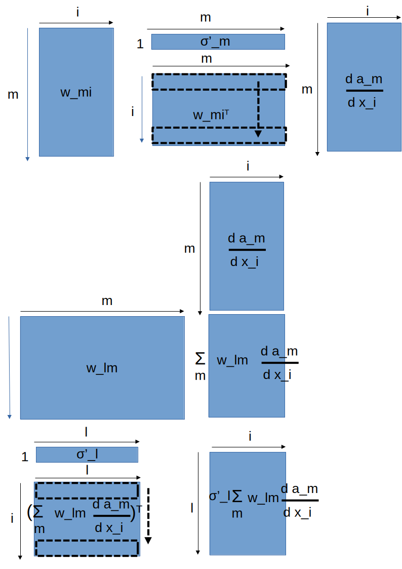
Jacobian

3. The only trick is to start by the jacobian variable with the identity matrix, this way every layer is treated the same way:

   • weights dot current jacobian

   • transpose

   • broadcast the activation derivative

   • transpose back

   • repeat

Exercise (difficult)

The goal is to implement the to following methods:

src

    def parameter_gradient(
        self, inputs: Sequence[Vector], targets: Sequence[Vector]
    ) -> tuple[list[Array2D], list[Vector]]:
        """The loss gradient with respect to the parameters: either weights or biases.

        dJ/dz of the last layer is first calculated.
        The detail of this computation depends on the loss function itself: usually
        either multi-class or regression. It is performed in the last_layer_dJdz method.

        The dJdz of the last layer allows to obtain the dJdb and dJdw of the last layer:
        dJ/dw_jk = dJ/dz_j a_k  with index k on the left and j on the right
        (which can be obtained by broadcast
                    a_0 ... a_k ...
        dJ/dz_0
        ...
        dJ/dz_j
        ...
        )

        Then, using back-propagation, every layer can be obtained from one before last to first:
        dJ/dw_kl = [ sum_j [w_jk s'(z_k) ] dJ/dz_j ] a_l  with index k on the left and j on the right

        c_jk = w_jk s'(z_k) simple broadcasting

        sum_j c_jk  dJ/dz_j is almost a dot product, requires a transpose -> d = c^T . dJ/dz

        dJ/dw_kl = c_k a_l can be obtained by broadcast similar as the one for the last layer

        At the end, the sum of the gradients for every case of the train set is divided by
        the number of cases of the train set to get the average gradient.
        """
        ...

src

    def fit(
        self,
        inputs: Sequence[Vector],
        targets: Sequence[Vector],
        learning_rate: float = 0.1,
        nb_iter_gradient: int = 1_000,
        regularization: float = 0.0,
    ) -> None:
        """Gradient descent algorithm on both the weights and biases, no stopping criteria,
        no stochastic pooling.

        The learning_rate is for the gradient from the train set.

        The regularization is the lambda_r of the basic regularization:
        J_r = lambda_r/2 (sum_all w^2 + sum_all b^2)
        """
        ...

The first implements the back-propagation algorithm; the second the gradient descent algorithm. Do not bother to implement a stopping criteria in the gradient descent, use a fixed number of iterations. Do not bother to implement stochastic gradient descent either. Some helper methods may help to factorize and shorten the code:

src

    def init_parameters_gradient_zero(self) -> tuple[list[Array2D], list[Vector]]:
        """initialize the arrays for the weight and biases gradients to zero
        with the correct dimension to be able to compute the mean gradients
        accross the train set."""
        ...

src

    def get_layer_activation_activation_derivative(
        self, ind_layer: int
    ) -> tuple[Layer, FuncVector, FuncVector]:
        """helper function, code factorisation"""
        ...

src

    def get_left_a_or_input(self, ind_layer: int, input_: Vector) -> Vector:
        """helper function, the FNN does not own the input,
        but uses it when left nodes of the first layer are required for an operation"""
        ...

Finally, to adapt for regression or multi-class classification:

src

    @staticmethod
    def last_layer_dJdz(
        layer: Layer,
        activation: FuncVector,
        activation_derivative: FuncVector,
        target: Vector,
    ) -> Vector:
        """Depending on the last layer activation, one assumes the loss is:
        + multi-class cross entropy for softmax
        + mean square error for linear"""
        ...

Hints 1

Start by drawing by hand every operation involved in the back-propagation clearly showing transpose, matrix multiplication and broadcast.

The back-propagation goes from last layer to first layer. The trick is to propagate the successive \(\cfrac{\partial J}{\partial z}\).

Treat the last layer separately to get the \(\cfrac{\partial J}{\partial z_j}\) in last_layer_dJdz; you can use the last layer activation to determine if this is a regression or a multi-class classification.

For the multi-class classification case the target which one-hot encoded makes the \(\cfrac{\partial J}{\partial z_j}\) easy to implement with an element-wise operation.

To compute the mean gradient for every training example, a loop over this examples and some arrays and vectors to cumulate all the individual gradients are useful.

Hints 2

\(\cfrac{\partial J}{\partial z_j}\) is an element-wise operation between 2 Vector (that is the reason why the activations and activation derivatives were implemented vectorized).

\(\cfrac{\partial J}{\partial w_{jk}}\) is a broadcast between a vertical 1 column 2d array and a 1d vector \(a_k\) in order to get the \(k\) index along the column. The result is a Array2d.

Hints 3

The \(\cfrac{\partial J}{\partial z_k}\) operation is a matrix product between a matrix \(w_{jk} \cdot\sigma'(z_k)\) and the vector \(\cfrac{\partial J}{\partial z_j}\) which has just been calculated previously. The operation \(w_{jk} \cdot\sigma'(z_k)\) is a simple broadcast.

The operation \(\cfrac{\partial J}{\partial w_{kl}}\) is similarly as previous hint, a broadcast between a vertical 1 column 2d array and a 1d vector \(a_l\) in order to get the \(l\) index along the column. The result is a Array2d.

Correction

src

    def init_parameters_gradient_zero(self) -> tuple[list[Array2D], list[Vector]]:
        """initialize the arrays for the weight and biases gradients to zero
        with the correct dimension to be able to compute the mean gradients
        accross the train set."""
        biases_all: list[Vector] = []
        weights_all: list[Array2D] = []
        # init to zero for cumsum over training examples
        for ind_layer in range(0, self.nb_layers):
            layer = self.layers[ind_layer]
            weights_all.append(
                np.zeros((layer.nb_nodes_right, layer.nb_nodes_left), dtype=FLOAT)
            )
            biases_all.append(np.zeros(layer.nb_nodes_right, dtype=FLOAT))
        return weights_all, biases_all

src

    def get_layer_activation_activation_derivative(
        self, ind_layer: int
    ) -> tuple[Layer, FuncVector, FuncVector]:
        """helper function, code factorisation"""
        layer: Layer = self.layers[ind_layer]
        activation: FuncVector = self.activations[ind_layer]
        activation_derivative: FuncVector = self.activation_derivatives[activation]
        return layer, activation, activation_derivative

src

    def get_left_a_or_input(self, ind_layer: int, input_: Vector) -> Vector:
        """helper function, the FNN does not own the input,
        but uses it when left nodes of the first layer are required for an operation"""
        return input_ if ind_layer == 0 else self.layers[ind_layer - 1].a

src

    @staticmethod
    def last_layer_dJdz(
        layer: Layer,
        activation: FuncVector,
        activation_derivative: FuncVector,
        target: Vector,
    ) -> Vector:
        """Depending on the last layer activation, one assumes the loss is:
        + multi-class cross entropy for softmax
        + mean square error for linear"""
        error: Vector = layer.a - target
        if activation == softmax:  # multi-class cross entropy gradient
            dJdz: Vector = error * target
        elif activation == linear:  # regression mean square gradient
            dJdz: Vector = error
        else:  # regression mean square gradient, other activations
            dJdz: Vector = error * activation_derivative(layer.z)
        return dJdz

src

    def parameter_gradient(
        self, inputs: Sequence[Vector], targets: Sequence[Vector]
    ) -> tuple[list[Array2D], list[Vector]]:
        """The loss gradient with respect to the parameters: either weights or biases.

        dJ/dz of the last layer is first calculated.
        The detail of this computation depends on the loss function itself: usually
        either multi-class or regression. It is performed in the last_layer_dJdz method.

        The dJdz of the last layer allows to obtain the dJdb and dJdw of the last layer:
        dJ/dw_jk = dJ/dz_j a_k  with index k on the left and j on the right
        (which can be obtained by broadcast
                    a_0 ... a_k ...
        dJ/dz_0
        ...
        dJ/dz_j
        ...
        )

        Then, using back-propagation, every layer can be obtained from one before last to first:
        dJ/dw_kl = [ sum_j [w_jk s'(z_k) ] dJ/dz_j ] a_l  with index k on the left and j on the right

        c_jk = w_jk s'(z_k) simple broadcasting

        sum_j c_jk  dJ/dz_j is almost a dot product, requires a transpose -> d = c^T . dJ/dz

        dJ/dw_kl = c_k a_l can be obtained by broadcast similar as the one for the last layer

        At the end, the sum of the gradients for every case of the train set is divided by
        the number of cases of the train set to get the average gradient.
        """
        # first store the sum for all training example of gradients
        # then at the end, the mean gradient
        gradients_weights: list[Array2D]
        gradients_biases: list[Vector]
        gradients_weights, gradients_biases = self.init_parameters_gradient_zero()

        for input_, target in zip(inputs, targets):
            # update all a and z for given training example
            self.infer(input_)

            ## last layer
            ind_layer = self.nb_layers - 1
            layer, activation, activation_derivative = (
                self.get_layer_activation_activation_derivative(ind_layer)
            )
            left: Vector = self.get_left_a_or_input(ind_layer, input_)

            dJdz: Vector = self.last_layer_dJdz(
                layer, activation, activation_derivative, target
            )

            gradients_biases[ind_layer] += dJdz
            dJdw: Array2D = dJdz[:, np.newaxis] * left  # broadcast
            gradients_weights[ind_layer] += dJdw

            dJdz_prev = dJdz

            ## layers from one before last included, to first
            for ind_layer in range(self.nb_layers - 2, -1, -1):
                layer, _, activation_derivative = (
                    self.get_layer_activation_activation_derivative(ind_layer)
                )
                left: Vector = self.get_left_a_or_input(ind_layer, input_)
                dJdz = (
                    self.layers[ind_layer + 1].weights
                    * activation_derivative(layer.z)  # broadcast
                ).T.dot(dJdz_prev)

                gradients_biases[ind_layer] += dJdz
                dJdw = dJdz[:, np.newaxis] * left  # broadcast
                gradients_weights[ind_layer] += dJdw

                dJdz_prev = dJdz

        # from sum to average
        nb_training = len(inputs)
        for ind_layer in range(0, self.nb_layers):
            gradients_weights[ind_layer] /= nb_training
            gradients_biases[ind_layer] /= nb_training

        return gradients_weights, gradients_biases

src

    def fit(
        self,
        inputs: Sequence[Vector],
        targets: Sequence[Vector],
        learning_rate: float = 0.1,
        nb_iter_gradient: int = 1_000,
        regularization: float = 0.0,
    ) -> None:
        """Gradient descent algorithm on both the weights and biases, no stopping criteria,
        no stochastic pooling.

        The learning_rate is for the gradient from the train set.

        The regularization is the lambda_r of the basic regularization:
        J_r = lambda_r/2 (sum_all w^2 + sum_all b^2)
        """
        if self.bad_input_or_target_size(
            self.nb_nodes_per_layer_including_input[0], inputs
        ):
            raise IncompatibleDimensions("The size of the input is incompatible.")
        if self.bad_input_or_target_size(
            self.nb_nodes_per_layer_including_input[-1], targets
        ):
            raise IncompatibleDimensions("The size of the target is incompatible.")

        for _ in range(nb_iter_gradient):
            gradients_weights, gradients_biases = self.parameter_gradient(
                inputs, targets
            )
            for ind_layer in range(self.nb_layers):
                self.apply_regularization(regularization)
                self.layers[ind_layer].weights -= (
                    learning_rate * gradients_weights[ind_layer]
                )
                self.layers[ind_layer].biases -= (
                    learning_rate * gradients_biases[ind_layer]
                )