Markov Decision Process
Definitions
A Markov Decision Process (MDP) is a mathematical framework used to model decision-making in environments where outcomes are partially random and partially under the control of a decision-maker. It serves as the formal foundation for Reinforcement Learning (RL), providing a structured way to describe how an agent interacts with a system over time to achieve a specific goal.
To define an MDP, you typically use four primary elements:
States (\(S\)): A set of all possible configurations or situations the system can be in (for example, the position and velocity of a mechanical arm).
Actions (\(A\)): The choices available to the decision-maker in each state (for example, applying a specific amount of torque). An action \(a\) may lead to a change of state from \(s\) to \(s'\).
Rewards (\(R\)): The immediate feedback \(r\) received after an action, used to signal whether an action was beneficial. The simplified case is when the reward is deterministic \(R(s'|s, a)\) (fixed for a transition between the current state \(s\) and the next state \(s'\)). However, sometimes the reward is stochastic (it fluctuates randomly following a distribution associated to the transition to the next state \(s'\) from the current state \(s\) when the action \(a\) is taken).
Transition Probability (\(T\)): The simplified definition is the probability that taking action \(a\) in state \(s\) will result in moving to state \(s'\). To be more explicit, this transition can be noted \(T(s'|s, a)\) as the probability to reach \(s'\) knowing \(s\) and \(a\). However, in the case of stochastic rewards, one uses the joint probability \(T(s', r|s, a)\) as the probability to reach \(s'\) and collecting \(r\) knowing \(s\) and \(a\): \(\sum_{s', r} T(s', r|s, a) = 1\).
A MDP is typically represented as a graph with two types of nodes: state nodes and chance|action nodes as illustrated on the Figure below. From a state node (blue ellipses), one or several actions are possible, taking an action (red arrow) moves you to the chance node (gray diamond). From the chance node, you randomly end up on a state node following the transition probability and collecting the reward. A reward can be seen as the opposite of a cost. A special state is the end state \(s_{\textrm{end}}\) from which no action can be performed and the process stops.
For a deterministic agent behavior, a policy \(\pi(s)\) defines the action \(a\) the agent will take for every state \(s\). However, the agent may behave stochastically. In this case, the policy defines for every state \(s\) the probability to take an action \(a\) and would be noted \(\pi(a | s)\). For example, the agent may choose its actions completely randomly: at every state it picks randomly an action in the set of available actions.
The value \(V_\pi(s)\) of a policy is the expected discounted sum of rewards collected following this policy \(\pi\) from state \(s\) until an end state is reached. Usually, the goal is to find an optimum policy: a policy with the maximum value. Since an immediate reward is sometimes preferred to a future reward, a discount factor \(\gamma\) (between 0 and 1) is used to weight down future rewards.
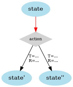
MDP structure
Exercise (easy)
This exercise is inspired from CS221 [LS]. Imagine a game, you are either “in” or “out”. In the later case, the game is ended. If you are “in”, you can either “quit” or “stay”. On one hand, if you choose to quit, you collect a reward of 10€ and the game is ended. On the other hand, you choose to stay, you role a die and you have a 2/3 probability to collect 4€ and be able to play again, and a 1/3 probability to be kicked out or the game and collect 5€. Draw the MDP graph of this game
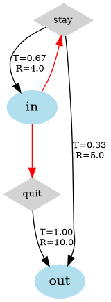
Exercise (easy)
For deterministic rewards and agent:
What python structure would you use to communicate a MDP assuming that the states and actions are
str? Fill it with the values corresponding to the game of the previous exercise.Same question for a policy?
For stochastic rewards and agent:
Same as 1.
Same as 2.
Correction
There is obviously not a unique answer:
State s |
||||
|---|---|---|---|---|
Action a |
||||
NextState s’ |
||||
Transition T |
Reward r |
|||
NextState s’’ |
||||
Transition T’ |
Reward r’ |
|||
Action a’ |
… |
For every state, potentially several actions are available. For each action, several next state are possible with a given transition / reward.
1type State = str
2type Action = str
3type NextState = str
4type Reward = float
5type Transition = float
6type Outcomes = dict[NextState, tuple[Transition, Reward]]
7
8type MDPMapping = dict[State, dict[Action, Outcomes]]
{'in': {'quit': {'out': (1.0, 10.0)},
        'stay': {'in': (2.0/3.0, 4.0), 'out': (1.0/3.0, 5.0)}},
'out': {}}
State s |
Action a |
State s’ |
Action a’ |
A deterministic policy tells you the action to perform for every state.
type PolicyMapping = dict[State, Action]
State s |
||||
|---|---|---|---|---|
Action a |
||||
NextState s’ |
||||
Transition T |
Reward r |
|||
Transition T’ |
Reward r’ |
|||
NextState s’’ |
||||
Transition T’’ |
Reward r’’ |
|||
… |
Note that now, the rewards are stochastic. It means that you have different probabilities for different rewards for a given (state, action to next state) case.
type Outcomes = dict[NextState, tuple[tuple[Transition, Reward], ...]]
State s |
||
Proba π |
Action a |
|
Proba π’ |
Action a’ |
|
State s’ |
||
Proba π’’ |
Action a’’ |
Note that the policy is now stochastic. It means that for each state you have a distribution of potential actions.
type ActionProbability = float
type PolicyMapping = dict[State, tuple[tuple[ActionProbability, Action], ...] ]
Policy value
Exercise (easy)
Preliminary question, imagine you play with a die (6 faces). You have one throw. If you get 1 or 2, you win 1€; 3, you win 10€; 4, 5, 6, you win 4€. What is the expected gain?
Correction
From a given state \(s\), several states \(s'\) are reachable following action \(a\) from the policy \(\pi\). Each one has a transition \(T(s' | s, a)\) and a reward \(R(s' | s, a)\). As a result, each next state \(s'\) contributes \(T(s' | s, a) R(s' | s, a)\) to the expected value \(V_\pi(s)\) of state \(s\) following \(\pi\). However, one must also account for the remaining value \(V_\pi(s')\) of every next state \(s'\): \(\gamma T(s' | s, a) V_\pi(s')\) (the \(\gamma\) is discounting the value \(V_\pi(s')\) because this value is one step in the future, and currents rewards are more valuable than future rewards).
For a deterministic policy, the value of a state \(s\) following a policy \(\pi\) is:
It is useful for later to define the quality \(Q_\pi(s, a)\) as the expected value from state \(s\) after action \(a\):
For a stochastic policy:
Exercise (intermediate)
For the game of the first exercise, calculate by hand the value of the policy “always play” assuming a discount value of 1.
Calculate by hand the value of the random policy \(\pi\), and all the qualities.
Correction
Applying the equations above:
(4)¶\[ \begin{align}\begin{aligned}V_\textrm{stay}(\textrm{in}) = \underbrace{\cfrac{1}{3} (5 + 0)}_{\textrm{next state: out}} + \underbrace{\cfrac{2}{3} \left( 4 + V_\textrm{stay}(\textrm{in}) \right)}_{\textrm{next state: in}}\\V_\textrm{stay}(\textrm{in}) \left( 1 - \cfrac{2}{3} \right) = \cfrac{13}{3}\\V_\textrm{stay}(\textrm{in}) = 13\end{aligned}\end{align} \]Obviously, it is not always possible to solve directly the recursive equation of the value. Next sections will present a general algorithm to do so.
One must distinguish clearly the value of the random policy from the quality of the policy when a specific action has been taken from a state:
(5)¶\[ \begin{align}\begin{aligned}V_\pi(\textrm{in}) = \cfrac{1}{2} \left( Q_\pi(\textrm{in}, \textrm{stay}) + Q_\pi(\textrm{in}, \textrm{quit}) \right)\\Q_\pi(\textrm{in}, \textrm{stay}) = \underbrace{\cfrac{1}{3} (5 + 0)}_{\textrm{next state: out}} + \underbrace{\cfrac{2}{3} \left( 4 + V_\textrm{stay}(\textrm{in}) \right)}_{\textrm{next state: in}} = \cfrac{13}{3} + \cfrac{2}{3} V_\pi(\textrm{in})\\Q_\pi(\textrm{in}, \textrm{quit}) = 10\\V_\pi(\textrm{in}) = \cfrac{1}{2} \left( \cfrac{13}{3} + \cfrac{2}{3} V_\pi(\textrm{in}) + 10 \right) = \cfrac{43}{4}\\Q_\pi(\textrm{in}, \textrm{stay}) = \cfrac{13}{3} + \cfrac{2}{3} \cfrac{43}{4} = \cfrac{23}{2}\end{aligned}\end{align} \]
Optimum policy
As mentioned, the next obvious step is to determine the optimum policy. The optimum policy is the mapping of actions per state which leads to the maximum expected value. For the type of MDP considered here, the optimum policy \(\pi_\textrm{opt}(s)\) is deterministic: for every state there is one action which will lead to the maximum value. As a result, the stochastic policy notation is dropped. For notation convenience, deterministic rewards are considered.
For every available action \(a\) from state \(s\), the optimum policy consists in choosing the action leading to a maximum value:
Algorithms
Hint
Equations (1) and (6) have a form: \(x=F(x)\) where the unknown \(x\) is the value. You already encountered this type of equations and numerically solved it iteratively using the by initializing the unknown at step \((0)\), and then improving until convergence the value of \(x^{((k+1))}\) from \(x^{((k))}\):
Policy evaluation
An algorithm to solve Equation (1) for every state is called policy evaluation:
1get all states
2initialize the value for all states to 0
3until convergence
4    for all states
5        calculate the quality for the current state ...
6        ... and the action from the policy using the current estimates of values for the next states
7        update the value of the current state
8    check convergence
Exercise (easy)
For the game of the first exercise, use the previous algorithm by hand to evaluate the policy “always stay” assuming a discount value of 1.
Same question for the random policy.
Correction
For always play:
which leads to the first ten values:
step |
V |
|---|---|
0 |
0.00 |
1 |
4.33 |
2 |
7.22 |
3 |
9.15 |
4 |
10.43 |
5 |
11.29 |
6 |
11.86 |
7 |
12.24 |
8 |
12.49 |
9 |
12.66 |
and ultimately a convergence towards the exact value which is 13.
For random policy:
which converges towards 43/4.
Value iteration
An algorithm to solve Equation (6) is called value iteration:
 1get all states
 2initialize the value for all states to 0
 3until convergence
 4    for all states
 5        for all actions at the current state
 6            calculate the qualities for the current state ...
 7            ... and the current action using current estimates of values for the next states
 8        update the value of the current state with the maximum quality between actions
 9        update the policy for the current state with the action giving the maximum quality
10    check convergence
Exercise (easy)
For the game of the first exercise, use the previous algorithm by hand to find the optimum policy assuming a discount value of 1.
Correction
Careful, one uses the current value of the optimum policy, which can fluctuate during convergence:
In the three following examples (game, magic tram, swamp isle) of the next section, the problem definition and the solving algorithms will be clearly separated similarly as what was done for the state problems. The basic structure of the problem is very similar to the state model structure. The key differences are:
the notion of transition (the next state is not certain after an action)
one maximizes rewards instead of minimizing costs (purely conventional)
Let us base the problem definition on the following types:
Note
The Outcomes type differs from the Outcome type of the state problems precisely to account for transitions.
Instead of a simple pair (next state, cost), one has a mapping between next states and pairs (transition, reward)
 1"""types and protocol for mdp"""
 2
 3from typing import Protocol, override
 4from collections.abc import MutableMapping
 5from random import choice
 6
 7
 8type State = str | int | tuple[int, ...]
 9type Action = str
10type NextState = State
11type Reward = float
12type Transition = float
13type Outcomes[S] = MutableMapping[S, tuple[Transition, Reward]]
14
15type MDPMapping[S] = MutableMapping[S, MutableMapping[Action, Outcomes[S]]]
16type PolicyMapping[S] = dict[S, Action]
17type ValuesMapping[S] = dict[S, Reward]
18type QualitiesMapping[S] = dict[tuple[S, Action], Reward]
19
20
21class MDPProblem[S: State](Protocol):
22    def actions_from_state(self, state: S) -> set[Action]: ...
23
24    def outcomes_from_state_and_action(self, state: S, action: Action) -> Outcomes: ...
25
26    @property
27    def states(self) -> set[S]: ...
28
29    def is_end_state(self, state: S) -> bool: ...
30
31    def export_to_MDPMapping(self) -> MDPMapping[S]:
32        mdp = {}
33        for state in self.states:
34            mdp[state] = {}
35            for action in self.actions_from_state(state):
36                mdp[state][action] = self.outcomes_from_state_and_action(state, action)
37        return mdp
38
39
40class Policy[S: State](Protocol):
41    def action_from_state(self, state: S, actions: set[Action]) -> Action: ...
42
43    # actions are required for the random policy
44
45
46class RandomPolicy[S: State](Policy):
47    @override
48    def action_from_state(self, state: S, actions: set[Action]) -> Action:
49        return choice(tuple(actions))
If the MDP is defined explicitly from a mapping, the MDPProblem can be specified:
src¶1class MDPFromMapping[S: State](MDPProblem[S]): 2 def __init__(self, mdp: MDPMapping) -> None: 3 self.mdp = mdp 4 5 def actions_from_state(self, state: S) -> set[Action]: 6 if self.is_end_state(state): 7 return set() 8 return set(self.mdp[state].keys()) 9 10 def outcomes_from_state_and_action(self, state: S, action: Action) -> Outcomes[S]: 11 return dict(self.mdp[state][action]) 12 13 @property 14 def states(self) -> set[S]: 15 return set(self.mdp) 16 17 def is_end_state(self, state: S) -> bool: 18 return not self.mdp[state]