Recursion

This section and the following ones develop three fundamental approaches to algorithm design:

• recursion

• divide and conquer

• dynamic programming

The emphasis is on algorithmic reasoning rather than programming syntax:

• identify recursive structures

• formulate appropriate base cases

• distinguish recursion from divide and conquer

• recognize overlapping subproblems

• define dynamic programming states

• reason about algorithmic complexity

A useful guiding principle is to ask:

1. Can the problem be expressed using smaller instances of itself?

2. Are the resulting subproblems independent?

3. Do identical subproblems occur repeatedly?

The answers often suggest the appropriate algorithmic paradigm.

Definition

A recursive algorithm solves a problem by reducing it to one or more smaller instances of the same problem.

Every recursive algorithm requires:

• a base case, solved directly;

• a recursive case, reducing the problem size.

Correct recursive algorithms require both progress and termination.

During the descent phase, the problem is decomposed. During the return phase, partial solutions are combined.

Exercise (easy)

The canonical problem to introduce recursion is the computation of \(N!\).

1. Write the base case, the recursive case.

2. Implement and test.

Correction

1. \[\begin{split}\begin{cases} 0! = 1 \\ N! = (N-1)! \, N \end{cases}\end{split}\]
2. src

   def factorial(number: int) -> int:
       if number < 0:
           raise ValueError("negative in factorial")
       if number == 0:
           return 1
       return number * factorial(number - 1)
   

   tests

   @pytest.mark.parametrize("number", (0, 3, 9))
   def test_factorial(number: int) -> None:
       assert factorial(number) == math.factorial(number)
   

   tests

   def test_factorial_error() -> None:
       with pytest.raises(ValueError):
           factorial(-1)
   

Exercise (easy)

A method to evaluate the numerical value of a polynomial is described below. A sequence contains the polynomial coefficients. The coefficients are sorted in descending powers of the polynomial: the first coefficient \(A_n\) is for the highest power term \(x^n\).

\[\left( \underbrace{ \left( \underbrace{ \left( \underbrace{A_n} \right) \cdot x + A_{n-1} } \right) \cdot x + A_{n-2} }\cdots \right) \cdot x + A_0\]

1. Write the base case, the recursive case.

2. Implement and test.

Hint

The underbrace indicates successive return values of the function.

The function np.polyval does the same job as Horner’s method.

Correction

1. The sequence of coefficients is noted \(s\)

\[\begin{split}\begin{cases} \textrm{horner}([\emptyset], x) = 0 \\ \textrm{horner}(s_{\textrm{without last}} ,x) \cdot x + s_{\textrm{last}} \end{cases}\end{split}\]

2. Two possible implementations:

src

def horner(coefficients: list[float], abscissa: float) -> float:
    if not coefficients:
        return 0.0
    coefficients_next: list[float] = coefficients.copy()
    last: float = coefficients_next.pop()
    return horner(coefficients_next, abscissa) * abscissa + last

tests

@pytest.mark.parametrize(
    "coefficients, abscissa",
    (
        ([], 5.0),
        ([3.0, 5.0, -1.0], 3.0),
        ([-2.0, 7.0, 1.0, -1.0], 4.0),
    ),
)
def test_horner(coefficients: list[float], abscissa: float) -> None:
    assert pytest.approx(horner(coefficients, abscissa)) == np.polyval(
        coefficients, abscissa
    )

src

def horner_no_copy(coefficients_: list[float], abscissa: float) -> float:
    def horner_nested() -> float:
        if not coefficients:
            return 0.0
        last: float = coefficients.pop()
        return horner_nested() * abscissa + last

    coefficients = coefficients_.copy()
    return horner_nested()

tests

@pytest.mark.parametrize(
    "coefficients, abscissa",
    (
        ([], 5.0),
        ([3.0, 5.0, -1.0], 3.0),
        ([-2.0, 7.0, 1.0, -1.0], 4.0),
    ),
)
def test_horner_no_copy(coefficients: list[float], abscissa: float) -> None:
    assert pytest.approx(horner_no_copy(coefficients, abscissa)) == np.polyval(
        coefficients, abscissa
    )

Exercise (intermediate)

The Laplace expansion expresses the determinant of a matrix in terms of its minors. The minor \(M_{i,j}\) is defined to be the determinant of the \((n-1) \times (n-1)\) matrix that results from \(A\) by removing the \(i\) th row and the \(j\) th column.

For every \(i\), so just choose one arbitrarily the first row, one has the equality:

\[\det(A)=\sum _{j=1}^{n}(-1)^{i+j}a_{ij}M_{ij}\]

If you do not understand this definition, take a look at this example.

1. Write the base case, the recursive case.

2. Implement and test.

3. Complexity. Assuming it takes in average 2 s to compute the determinant of a matrix of size 10. How long will it take for a matrix of size 20?

Hint

Careful, the math index notation starts at 1 whereas python indexes start at 0.

The function np.linalg.det computes the determinant.

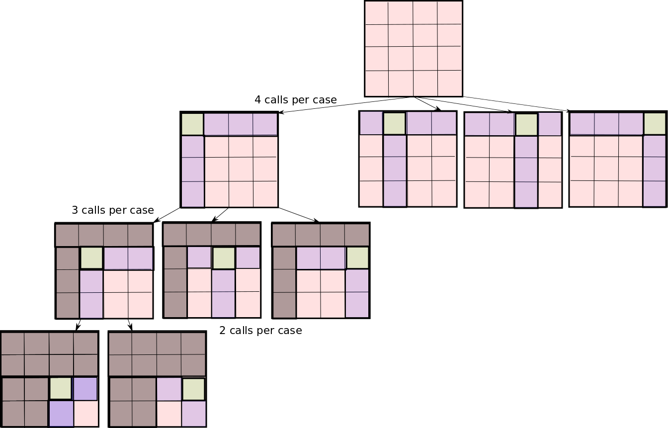
Determinant by Laplace expansion

Correction

\[\begin{split}\begin{cases} \det({\textrm{scalar}}) = \textrm{scalar} \\ \det(A) = \sum _{j=0}^{n-1}(-1)^{j}a_{0j} \det( A_{\textrm{without row 0 and column j}} ) \end{cases}\end{split}\]

import numpy as np
import numpy.typing as npt

type Matrix = npt.NDArray

src

def determinant(matrix: Matrix) -> float:
    """determinant by laplace expansion on the first row"""
    nb_rows, nb_columns = matrix.shape
    if nb_rows != nb_columns:
        raise ValueError("non square matrix in determinant")
    if nb_rows == 1:
        return matrix[0, 0]
    det: float = 0.0
    for ind_col in range(nb_rows):
        left: Matrix = matrix[1:nb_rows, :ind_col]
        right: Matrix = matrix[1:nb_rows, (ind_col + 1) :]
        det += (
            (-1) ** ind_col * matrix[0, ind_col] * determinant(np.hstack((left, right)))
        )
    return det

tests

def test_determinant() -> None:
    nb_rows = 5
    matrix = np.random.random((nb_rows, nb_rows))
    assert pytest.approx(determinant(matrix)) == np.linalg.det(matrix)

3. Remember that:

   \[e - 1 = \sum_{i=1}^\infty \cfrac{1}{i!}\]

   Let’s define the costly operation as the computation of \((-1)^{i+j}a_{ij}\) times the scalar value of whatever is the results of \(M_{ij}\). This does not include all the operations required to get this \(M_{ij}\). Here, \(M_{ij}\) is just seen as a scalar. This costly operation has a constant time which does not depend on the problem size. The idea is now to count as function of \(n\) the number of times this operation occurs.

   For a \(n\times n\) matrix, the first level of recursion makes \(n\) calls. At every call, the costly operation takes place. The second level of recursion makes \(n-1\) calls for each case of the first level of recursion. The third level makes \(n-2\) calls per case of level \(n-1\), and so on.

   At the deepest level of recursion the determinant of a scalar is the scalar itself. It terminates the chain of recursion. At this bottom level, \(M_{ij}\) is truly a scalar (the determinant of a scalar is himself).

   So, all things considered, you can just count the number of costly operations:

   \[\begin{split}\mathcal{n} &= n + n(n-1) + n(n-1)(n-2) + \cdots + n(n-1)\cdots4\times3 + n! \\ &= n! \underbrace{\left(\cfrac{1}{(n-1)!} + \cfrac{1}{(n-2)!} + \cfrac{1}{(n-3)!} + \cdots + \cfrac{1}{2} + 1\right)}_{ \textrm{asymptotically } e - 1}\end{split}\]

   It leads to a number of costly operations proportional to \(n!\). This would lead to a catastrophic explosion of computing time for larger and larger matrices.

   \[2\textrm{s} \times \cfrac{20!}{10!}\approx 40\,000 \textrm{years}\]

Exercise (intermediate)

Obtain all possible permutations of a sequence.

1. Write the base case, the recursive case.

2. Implement and test.

Hint

The recursive case needs some thinking. Our permutate function is expected to return every permutation of a given sequence. Thus, this function is able to return every permutation of the sequence without its last element. Assuming that your function works, and that you have at your disposal all the permutations of the sequence without its last element, how can you produce all the permutations possible with the last element?

Correction

1. The answer to the question in the hint above is: you just have to insert this element at every location possible, for every permutated sequence without the last element:

   • initial sequence [1, 2, 3]

   • all permutations without last elt [[1, 2]; [2, 1]]

   • all sequences produced by inserted 3 at every location [[3, 1, 2], [1, 3, 2], [1, 2, 3]; [3, 2, 1], [2, 3,1], [2, 1, 3]]

   The base case is obvious, for a empty sequence or a singleton, there is a single “permutation”: the original sequence.

src

def permutate[T](seq: list[T]) -> list[list[T]]:
    """all permutations of a sequence obtained:

    [x, y, z] drop last

    [ [x, y], [y, x] ] get every permutation of remaining

    insert last at every possible location
    [
        [z, x, y], [x, z, y], [x, y, z],
        [z, y, x], [y, z, x], [y, x, z]
    ]"""
    nb_elts: int = len(seq)
    if nb_elts <= 1:
        return [seq]

    seq_without_last_elt: list[T] = seq.copy()
    elt: T = seq_without_last_elt.pop()
    all_permutated_seqs_with_elt_at_every_location: list[list[T]] = []
    all_permutated_seqs_with_last_elt_missing: list[list[T]] = permutate(
        seq_without_last_elt
    )
    for permutated_seq in all_permutated_seqs_with_last_elt_missing:
        nb_insert_locations: int = len(permutated_seq) + 1
        for ind in range(nb_insert_locations):
            permutated_seq_with_elt_inserted = (
                permutated_seq[:ind] + [elt] + permutated_seq[ind:]
            )
            all_permutated_seqs_with_elt_at_every_location.append(
                permutated_seq_with_elt_inserted
            )
    return all_permutated_seqs_with_elt_at_every_location

tests

def test_permutate() -> None:
    seq: list[int] = list(range(5))
    assert {tuple(permutated_seq) for permutated_seq in permutate(seq)} == set(
        permutations(seq)
    )
    assert permutate([]) == [[]]

Exercise (intermediate)

Create a generator of the cartesian product of a sequence of iterables. Test it.

Correction

src

def cartesian_product[T](iterables: Sequence[Iterable[T]]) -> Generator[list[T]]:
    """yields every combination of element picked in an arbitrary number of iterables:
    [[1, 2], [3, 4]]

    [1, 3]; [1, 4]; [2, 3]; [2, 4]"""
    nb_iterables: int = len(iterables)

    def _nested_cartesian_product(
        product: list[T], index_iterable: int
    ) -> Generator[list[T]]:
        """product is one of the future yielded iterable under construction,
        an item is picked in the first, then assembled to an item picked in the second, etc

        until an item is picked in the last iterable, then the product can be yielded"""
        if index_iterable == nb_iterables:
            yield product
        else:
            for item in iterables[index_iterable]:
                yield from _nested_cartesian_product(
                    product + [item], index_iterable + 1
                )

    return _nested_cartesian_product([], 0)

tests

def test_cartesian_product() -> None:
    seqs: list[list[int]] = [list(range(5)), list(range(3)), list(range(4))]
    obtained = {tuple(seq) for seq in cartesian_product(seqs)}
    expected = {tuple(seq) for seq in product(*seqs)}
    assert obtained == expected
    assert list(cartesian_product([[]])) == []