Higher order derivatives
The previous section showed the basics of auto-differentiation. However, what one really need is to be able to differentiate at higher orders: either, second derivatives or cross-derivatives (coordinates and network parameters).
For the moment, one is able to encode an expression with forward operations, building a computation graph. Then, the backward sweep computes the numerical value of all intermediate derivatives. However, these numerical values are just numerical values. It is for the moment impossible to differentiate a second time or with respect to an other parameter. What is really required, is to build the computation graph of all the operations of the backward sweep.
It means that first, a computation graph of the initial expression is obtained during the first forward sweep. Then, all the backward operations must build another computation graph of all the operations required to obtain the first derivative. Next, this process can be once again repeated, by operating a backward sweep on the computation graph of the first derivative, building the computation graph of the second derivatives, and so on and so on.
Note
A backward sweep is just a succession of operations, its computation graph can be built. Then, additional backward sweeps can be performed starting from the nodes representing the derivatives in order to get higher order differentiation and cross-derivatives.
To be able to build the computation graph of a backward sweep, one has to remember the operations involved:
set the leaf node to one
go backward in a topological order
apply the backward operation and cumulate the intermediate result
repeat the last two steps
Let us take a trivial example:
The forward graph is:
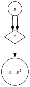
Forward sweep (higher)
For the backward sweep, the multiplication with one and the first cumulate with zero creates several useless operations (grey edges):
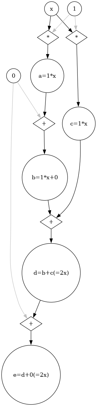
Backward sweep (higher)
Dropping the useless stuff:
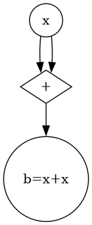
Simplifified first backward sweep (higher)
The second backward sweep gives:
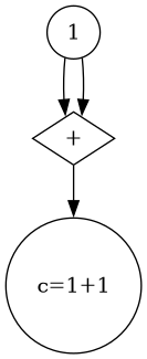
Simplifified second backward sweep (higher)
Finally, all the operations together:
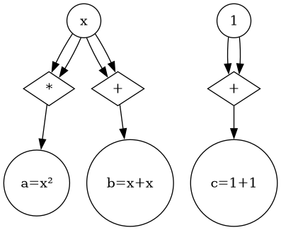
Overall (higher)
Example
A slightly less trivial example with a function of two variables (to see how cross-derivatives can be obtained):
The forward graph is:
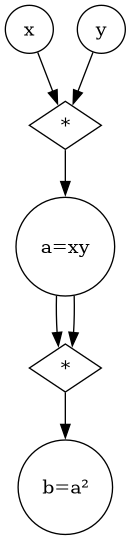
Forward sweep (higher)
Let us take this simple example, and list very pedantically every operation of the backward sweep. The previous edges are dashed.
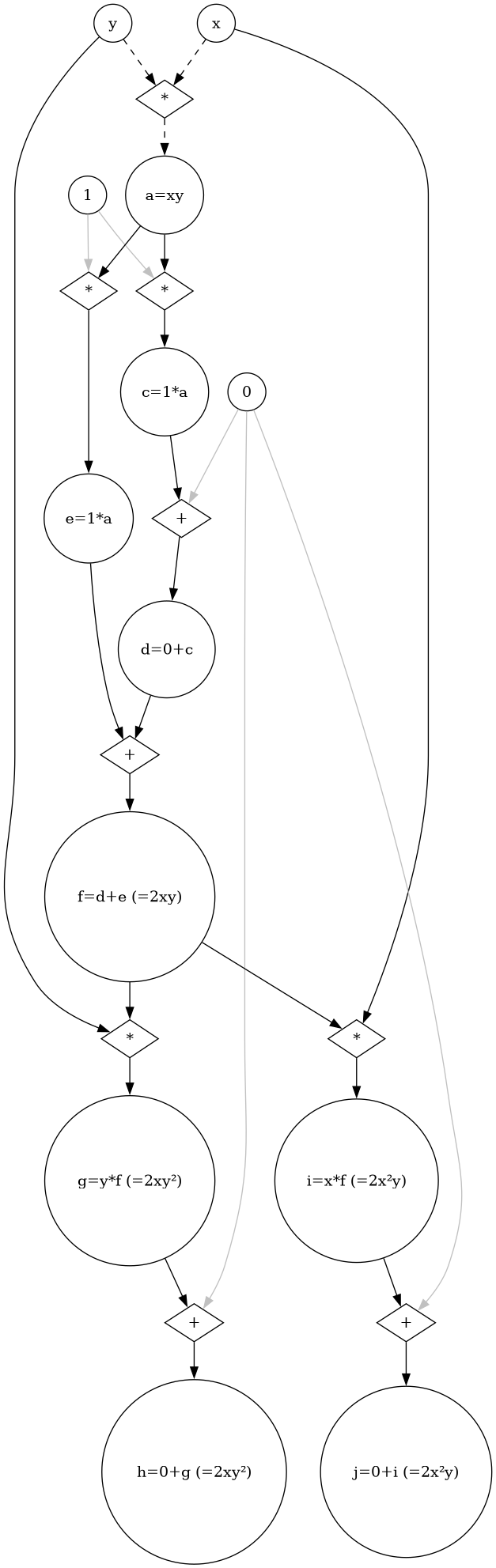
Backward sweep (higher)
To clarify, let us drop the multiplication by a constant \(1\) and the addition to a constant \(0\) which are the grey edges, one gets:
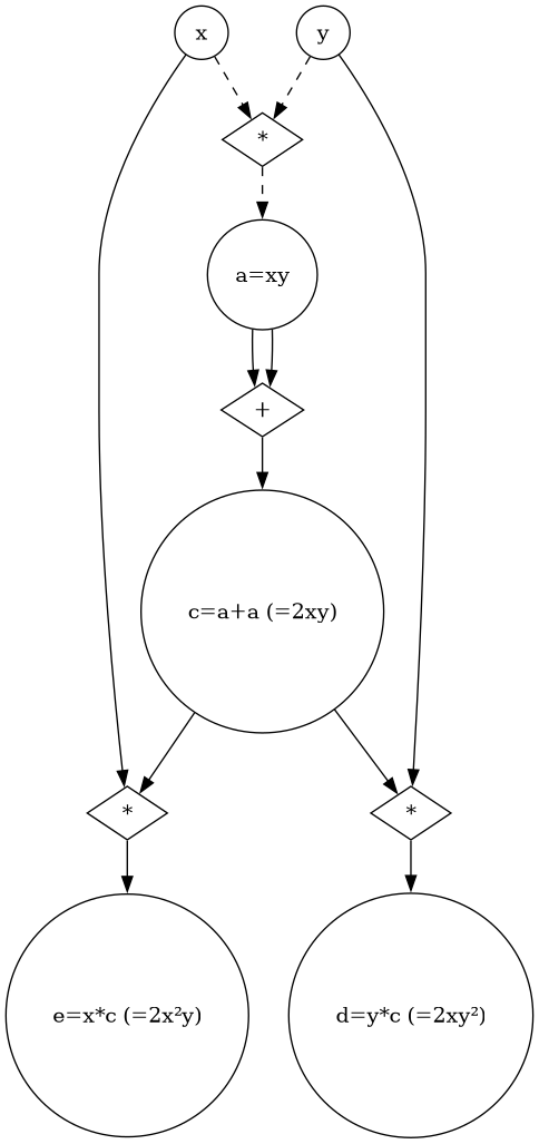
Backward sweep simplified (higher)
Starting from the node representing the \(\cfrac{\partial f}{\partial x}\) (d), a backward sweep is performed:
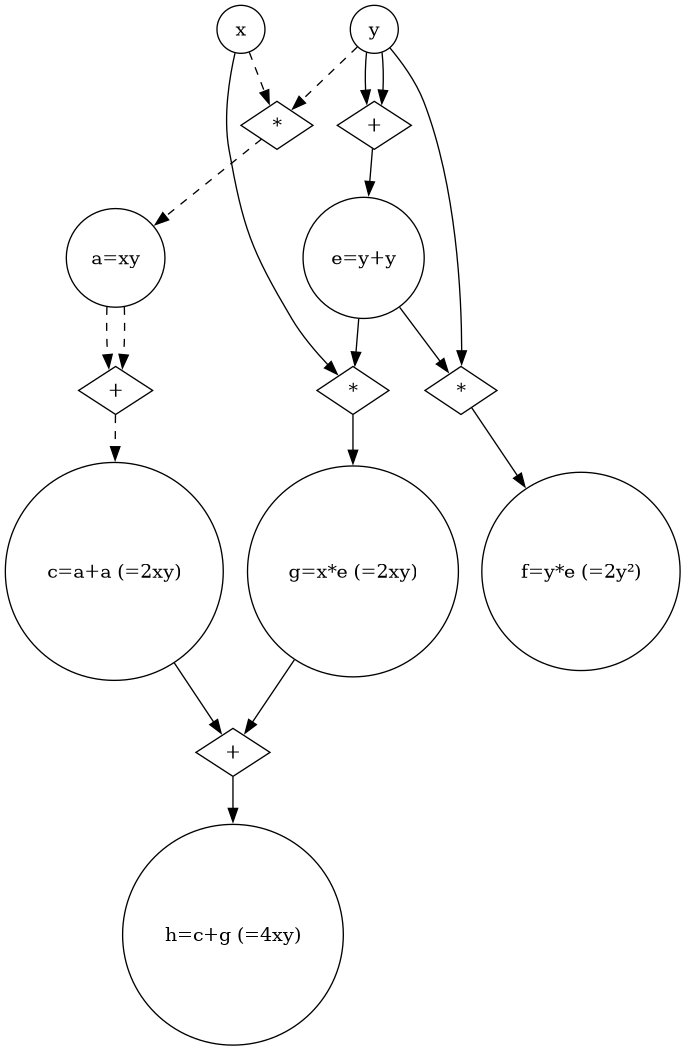
Second backward sweep simplified (higher)
If everything so far is put together, the overall computation graph is obtained. The bottom left red solid node is \(\cfrac{\partial f}{\partial x}\); the bottom right blue solid node is \(\cfrac{\partial f}{\partial y}\); the central left red dashed node is \(\cfrac{\partial^2 f}{\partial x^2}\); the bottom central purple dashed node is \(\cfrac{\partial^2 f}{\partial x \partial y}\);
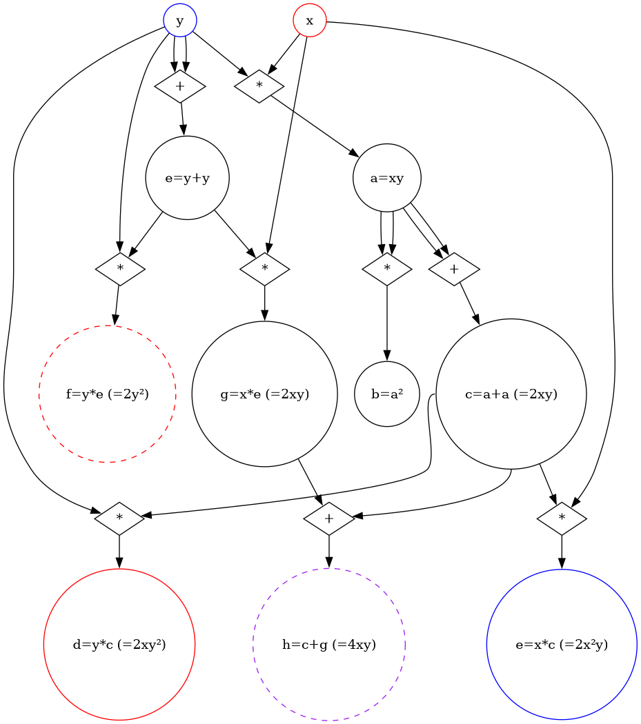
Overall (higher)
Implementation
As expected, even though the process is plain and systematic, it is very tedious.
Let us implement it.
The key point to grasp is that formerly, all the intermediate derivatives were just numerical values stored in a dict,
however from now on, all the operations leading to such derivatives are recorded in a computation graph.
It implies two major changes:
the derivative values become
Nodeinstead offloatthe operations used to calculate derivatives: the
backwardoperations, must now on use theforwardoperations in order to create the computation graph of every backward sweep.
 1@dataclass
 2class Node:
 3    val: float
 4    parents: tuple[Self, ...] = field(default_factory=tuple)
 5    name: str = ""
 6    operation: str = ""
 7    is_constant: bool = False
 8
 9    index: int = field(init=False)
10
11    _counter: ClassVar[int] = 0
12
13    def __post_init__(self) -> None:
14        self.backward: Backward = lambda _, __: None
15        self.index = self._counter
16        self._increment_counter()
17
18    def __hash__(self) -> int:
19        return self.index
20
21    @classmethod
22    def _increment_counter(cls):
23        cls._counter += 1
The attribute operation is there only for debugging purposes, as is the name.
The differentiate function is almost identical:
 1def differentiate(node: Node) -> Derivatives:
 2    """after getting the topological order,
 3    computes the numerical values of every intermediate
 4    derivatives by calling the backward callbacks of every node.
 5
 6    However, the difference with the first order differentiation is
 7    that the Derivatives dict is [Node, Node], instead of [Node, Float],
 8    building a computation graph during a reverse sweep.
 9
10    If the node is declared constant, all the derivatives are zero.
11    Using a defaultdict derivatives allows to return zero Node if a key is not present.
12
13    It serves two purposes:
14    - first the cumulate operation in the backward callbacks is automatically valid
15    - if a node is not key, it means it is not part of the parent tree,
16      so the derivative should be zero Node"""
17
18    order: tuple[Node, ...] = topological_sort(node)
19
20    def zero():
21        return ZERO
22
23    derivatives: dict[Node, Node] = defaultdict(zero)
24
25    if node.is_constant:
26        return derivatives
27
28    derivatives[node] = ONE
29    for current in order:
30        current.backward(current, derivatives)
31    return derivatives
Exercise (intermediate)
Implement and test the multiplication and addition backward operations.
Correction
1def multiplication_backward(node: Node, derivatives: Derivatives) -> None:
2    for ind in range(2):
3        if not node.parents[ind].is_constant:
4            derivatives[node.parents[ind]] = addition_forward(
5                multiplication_forward(node.parents[1 - ind], derivatives[node]),
6                derivatives[node.parents[ind]],
7            )
1def addition_backward(node: Node, derivatives: Derivatives) -> None:
2    for parent in node.parents:
3        if not parent.is_constant:
4            derivatives[parent] = addition_forward(
5                derivatives[parent], derivatives[node]
6            )
1@pytest.fixture(params=list(range(1, 4)))
2def x_val(request) -> float:
3    x_val = float(request.param)
4    return x_val
 1@pytest.fixture(params=list(range(2, 6)))
 2def x_pow_one_by_one(request, x_val) -> tuple[Node, Node, float, float, float]:
 3    max_power: int = request.param
 4    x = Node(x_val, name="x")
 5    z = x
 6    for _ in range(max_power - 1):
 7        z = multiplication_forward(z, x)
 8    return (
 9        x,
10        z,
11        x_val**max_power,
12        max_power * x_val ** (max_power - 1),
13        max_power * (max_power - 1) * x_val ** (max_power - 2),
14    )
 1@pytest.fixture(params=list(range(1, 6)))
 2def x_sum_one_by_one(request, x_val) -> tuple[Node, Node, float, float, float]:
 3    max_repet: int = request.param
 4    x = Node(x_val, name="x")
 5    z = x
 6    for _ in range(max_repet - 1):
 7        z = addition_forward(z, x)
 8    return (
 9        x,
10        z,
11        max_repet * x_val,
12        max_repet,
13        0.0,
14    )
 1def assert_derivatives(x_z_zv_dzv_d2zv: tuple[Node, Node, float, float, float]) -> None:
 2    x, z, z_val, dz_val, d2z_val = x_z_zv_dzv_d2zv
 3    print(f"\n x={x.val} f(x)={z.name}")
 4
 5    assert pytest.approx(z.val) == z_val
 6
 7    # ic(z)
 8    # breakpoint()
 9
10    dz: Derivatives = differentiate(z)
11    dzdx: Node = dz[x]
12
13    # ic(dz)
14    # breakpoint()
15
16    assert pytest.approx(dzdx.val) == dz_val
17
18    d_dzdx: Derivatives = differentiate(dzdx)
19    d2zdx2: Node = d_dzdx[x]
20
21    assert pytest.approx(d2zdx2.val) == d2z_val
1def test_derivatives_pow_one_by_one(x_pow_one_by_one):
2    assert_derivatives(x_pow_one_by_one)
1def test_derivatives_sum_one_by_one(x_sum_one_by_one):
2    assert_derivatives(x_sum_one_by_one)